Quick Start
This quick tutorial walks you through launching OpenIMC, loading an IMC file, visualizing channels, and running a basic segmentation workflow.
Launching OpenIMC
After installation, start the GUI by running:
openimc-gui
This opens the full OpenIMC interface.
Note
The command python -m openimc runs the CLI (command-line interface) for batch processing, not the GUI. Use openimc-gui to launch the graphical interface.
Basic Workflow
This section walks you through the essential steps of an IMC analysis workflow from file loading to spatial analysis.
Step 1: Open an IMC File
Select File → Open File/Folder, then choose the .mcd file(s) you want to analyze.
Multiple files can be selected using Shift or Ctrl.
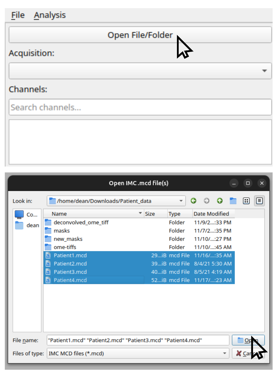
Figure 1: Selecting one or more .mcd files in the OpenIMC GUI.
Step 2: Explore the Image
Newly loaded files appear in the image viewer. By default, channels are shown in a grid layout.
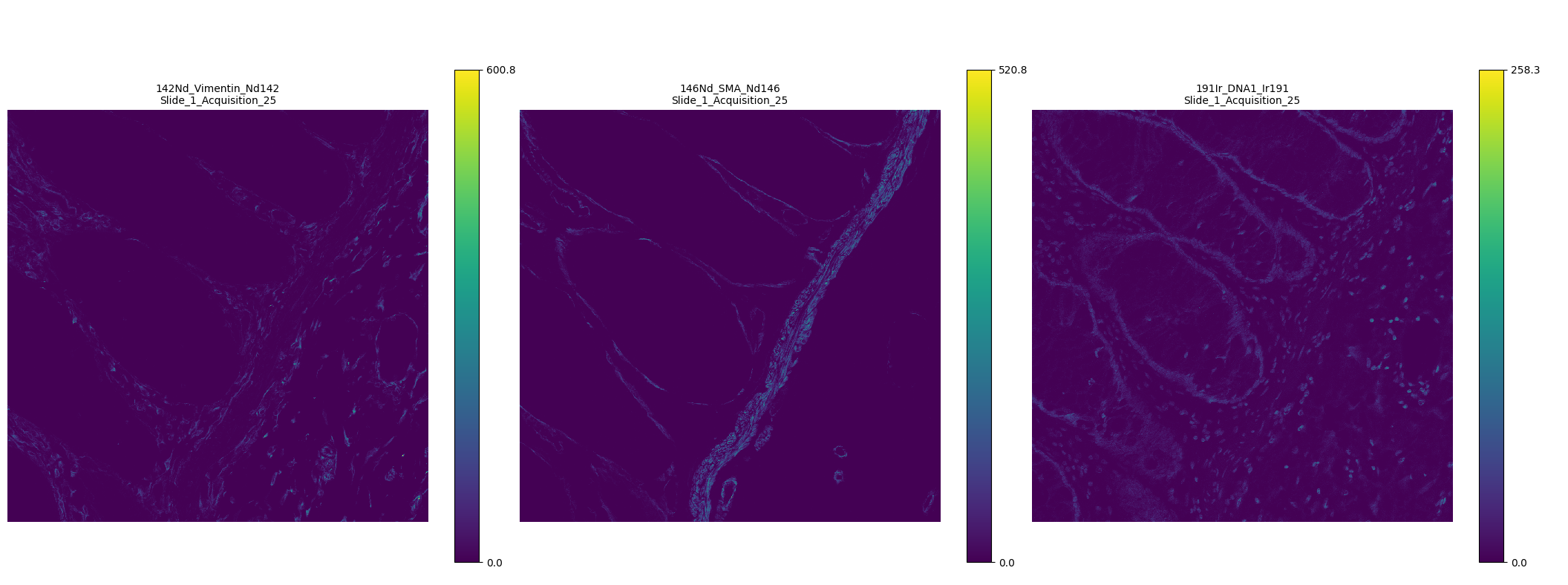
Figure 2: Grid-based visualization of multiple IMC channels.
Viewing Options:
Grayscale mode: Switch to grayscale by enabling Grayscale mode.
RGB composite view: To view channels as a composite RGB image, disable Grid view for multiple channels. A dropdown will appear to assign channels to R, G, and B. Composite intensity is computed using the selected merge method.
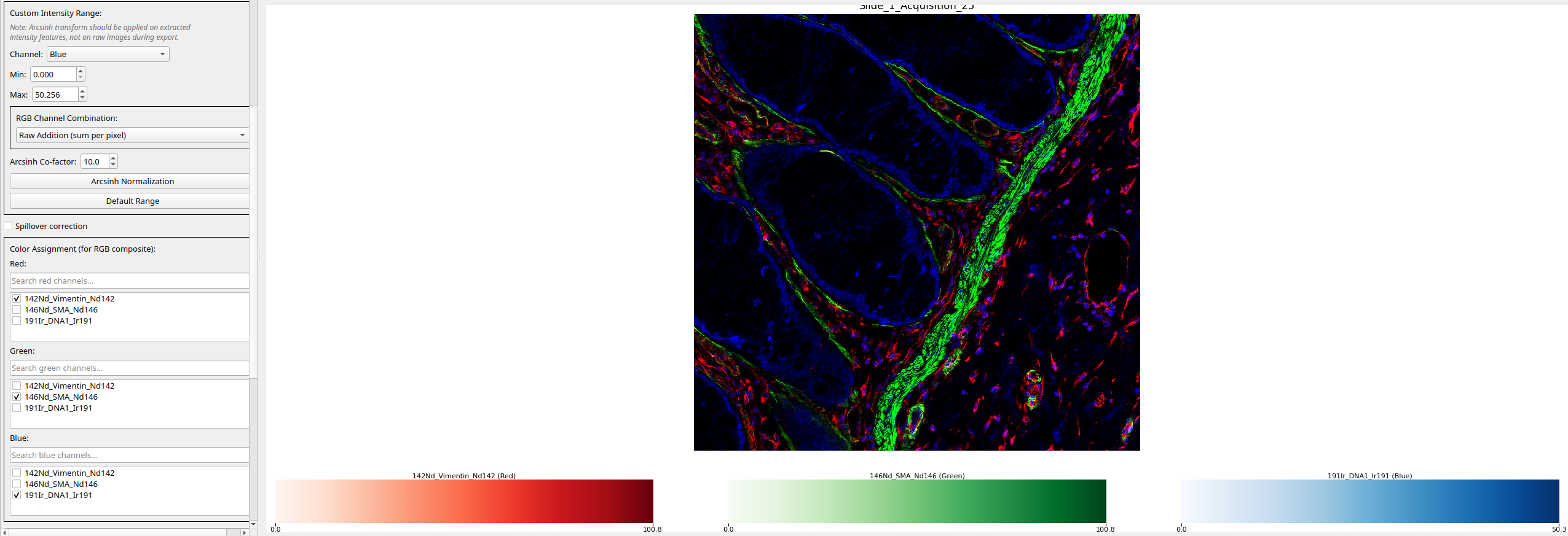
Figure 3: RGB composite view generated from user-selected channels.
Additional Tools:
Custom scaling: Interactively rescale intensities.
Scale bar: Add and configure a micrometer scale bar.
These options help you quickly assess signal quality, contrast, and cell morphology.
Step 3: Run Segmentation
Click Cell Segmentation to open the segmentation dialog. Choose a segmentation method and select the channels appropriate for your experiment.
Available Segmentation Engines:
DeepCell CellSAM
Cellpose cyto3 (cytoplasm + nucleus)
Cellpose nuclei model
Ilastik (
.ilpmodels)Watershed
Recommendations:
For most datasets, DeepCell CellSAM provides the best overall performance. DeepCell CellSAM is a transformer-based model and requires a GPU to run quickly (CPU still works, but will be slow). If you do not have a GPU, Cellpose is a potential alternative, but will still be slow on CPU.
CellSAM Configuration:
If using CellSAM, enter your DeepCell API token under DeepCell CellSAM Parameters. Adjustable CellSAM options:
Bbox threshold (default 0.4)
Use WSI mode (tiling for large images)
Low contrast enhancement
Gauge cell size
Note
Before segmenting an entire experiment, it is recommended to test on a single acquisition and refine settings.
Once segmentation completes, enable Show Overlay to visualize masks on top of any channel.
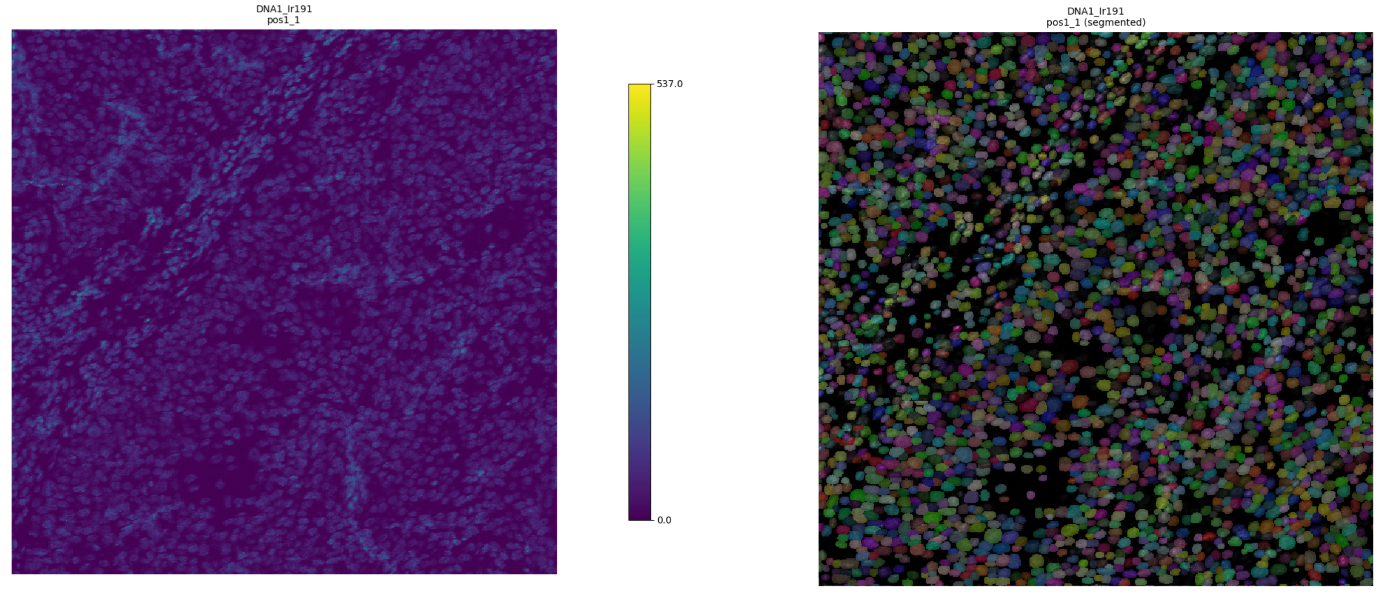
Figure 4: Segmentation mask overlaid on the DNA channel after processing with DeepCell CellSAM. Masks and the raw image are shown side by side.
Step 4: Extract Features
Click Feature Extraction to open the feature extraction dialog.
Primary Settings:
Acquisitions: The acquisitions to extract features from (default is all acquisitions with segmentation masks)
Output: The output directory for the features (default is the current directory)
Denoising: The denoising method to use (for most datasets, hot pixel removal by Median 3x3 is recommended, ensure you click ‘Apply to all channels’)
Arcsinh scaling: Whether to apply arcsinh scaling to the intensity features (for most datasets, this is recommended)
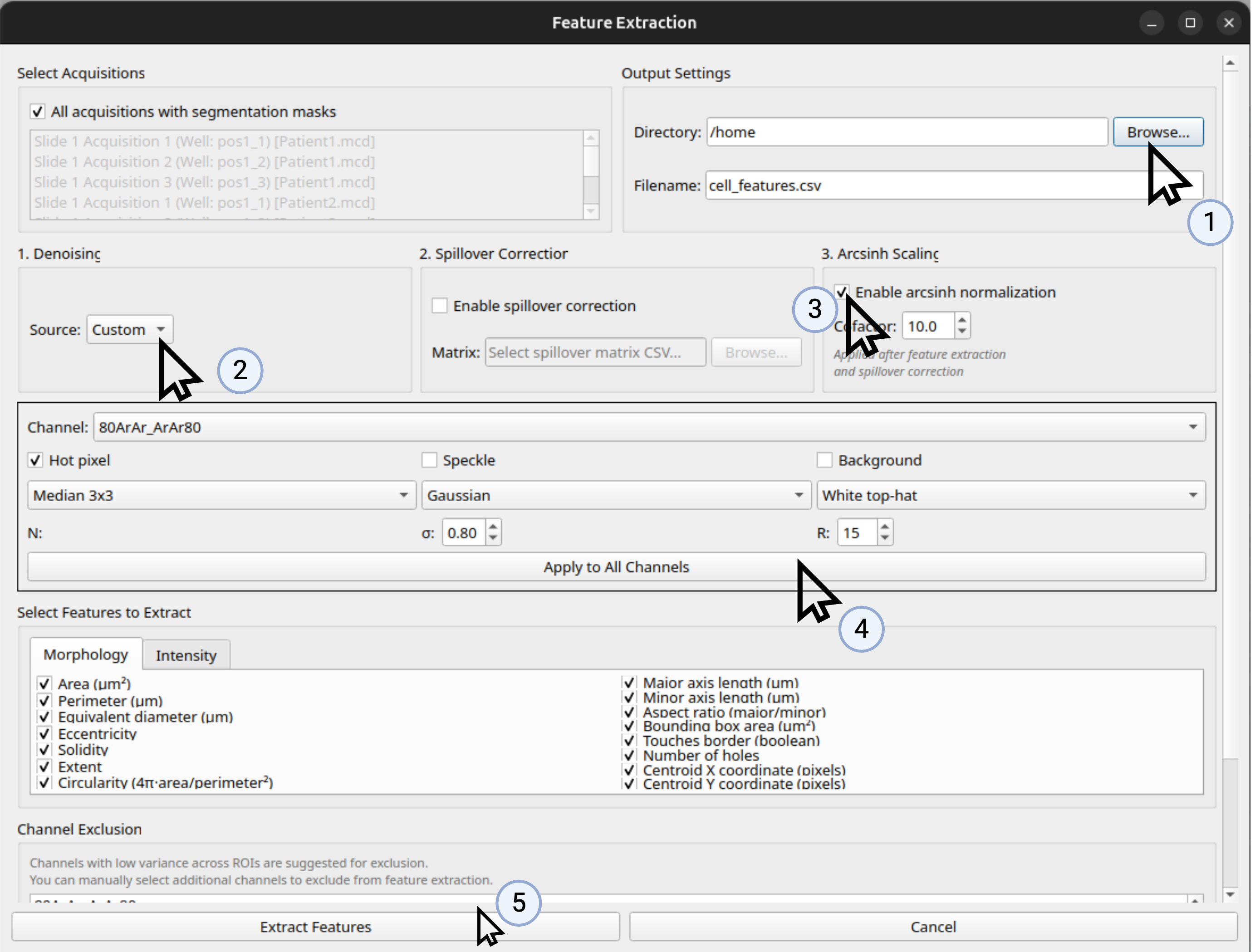
Figure 5: Recommended Settings for Feature Extraction for Most Datasets.
Click ‘Extract Features’ to start the feature extraction process. The features will be saved to the output directory as a CSV file. The data will continue to be stored in memory for further analysis, including clustering and spatial analysis, and does not need to be reloaded.
Step 5: Cluster Cells
Click Cell Clustering to open the clustering dialog. The features extracted from the previous step will be loaded automatically.
Selecting a Clustering Method
At the top of the clustering dialog, you can select the type of clustering to perform.
Available Clustering Methods:
Leiden
Louvain
Hierarchical
K-means
HDBSCAN
Method Recommendations:
Leiden and Louvain: Recommended for most datasets with high cell density and highly varying types of cells.
Hierarchical: Recommended for datasets with a small number of cells or a small number of cell types.
K-means: Recommended for datasets with approximately equal numbers of cells of each type.
HDBSCAN: Recommended for datasets with many outliers or cells that are not well-defined.
After selecting the clustering method, you can set the parameters for the clustering method. See the Clustering section for more details. For most datasets, the default settings will be sufficient.
Note
We recommend using Leiden clustering for most datasets.
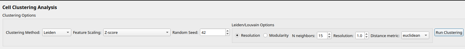
Figure 6: Clustering Dialog Settings, default to Leiden clustering.
Feature Selection
After you hit ‘Run Clustering’, a pop-up will ask you to select the features to cluster. Features will be subset to the mean intensities and the morphological features. At this stage, it is important to select the features that are most informative for the clustering. If you know that certain antibodies are not working well, you should exclude them from the clustering.
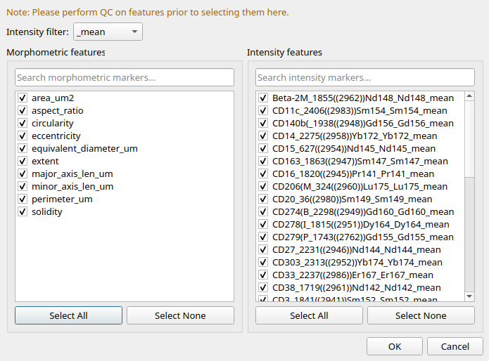
Figure 7: Feature Selection for Clustering.
Visualizing Clusters
Once the clustering is complete, you can visualize the clusters. The default visualization is a heatmap of the clusters.
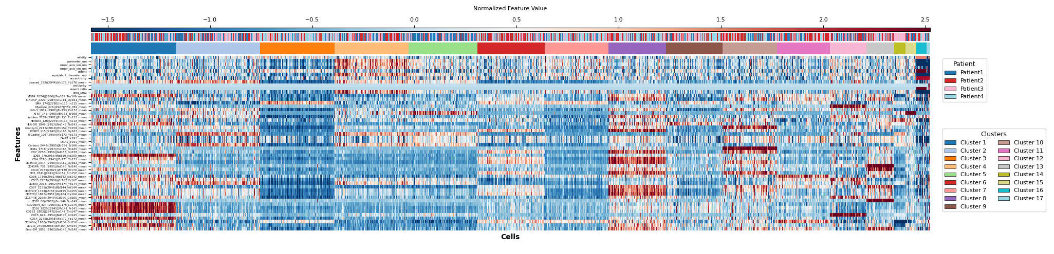
Figure 8: Heatmap of the clusters, with annotation of both the clusters and the patients from which the cells are derived.
Additional Visualization Options:
At the bottom of the clustering dialog, you can change to various other visualizations, including:
UMAPs
t-SNE
Stacked Bars
Differential Expression
Boxplot/Violin Plot
Saving Results:
Save the visualization as a PNG file by clicking the ‘Save Plot’ button.
Save the clustering output as a CSV file by clicking the ‘Save Clustering Output’ button. This will save the features with cluster labels and/or any manual annotations.
Step 6: Cell Phenotyping
After clustering, you can annotate the clusters by their cell type. This is done by clicking the ‘Annotate Phenotypes’ button.
Annotation Methods:
You can either:
Manually annotate the clusters by typing in the cell type name
Use the LLM to annotate the clusters
Using LLM Annotation:
The LLM will ask you for an OpenAI API key. If you do not have an OpenAI API key, you can get one by signing up for an account at https://openai.com/ (see the Installation section for more details).
You can also provide context to the LLM (such as the cancer type, the tissue type, the treatment, the patient metadata, etc.) This will help the LLM to generate more accurate cell type annotations.
Warning
The LLM is charged by the token, so ensure your account has enough credits.
Note
The LLM is not perfect, so you should manually check the annotations and correct them if necessary.
Once the LLM has suggested the cell types, you can choose from its suggestions and update your plot.
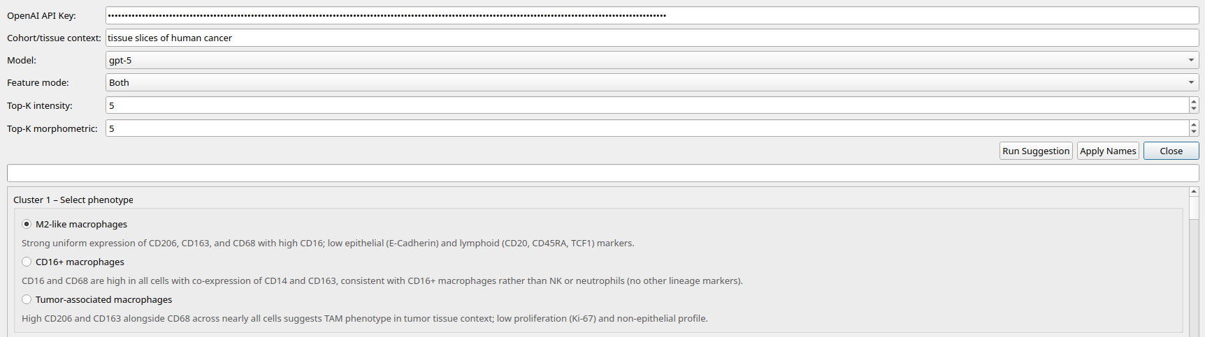
Figure 9: Phenotyping with ChatGPT suggestions.
Step 7: Spatial Analysis
After clustering, you can perform spatial analysis to investigate the spatial distribution of the cells. This is done by clicking the ‘Spatial Analysis’ button.
Analysis Modes:
Spatial analysis is split into two windows:
Simple analysis: For most users, this will be sufficient
Advanced analysis: For more complex spatial analyses
Building the Spatial Graph
The first step of spatial analysis is to build a spatial graph of the cells. There are three methods to build the spatial graph:
k-nearest neighbors (kNN): The default method and recommended for most datasets. K is the number of neighbors to consider for the spatial graph for each cell. Set this to a reasonable number based on the density of the cells.
Radius: Connect cells within a chosen radius. In the advanced Squidpy-backed workflow, radius is interpreted in micrometers after coordinate scaling; see the Simple Spatial Analysis page for the current simple-workflow radius semantics.
Delaunay: Recommended for datasets with a large number of cells or a large number of cell types. Delaunay is based on the Delaunay triangulation of the cells. See more details in the Spatial Analysis section.
Available Visualizations:
Some spatial visualizations are available in the simple analysis window, including:
Spatial visualization of the cells: Represent each cell as a point, color by their cluster, and show the edges between the cells
Distance distribution of the cells: Show the distance distribution of the cells by their cluster → what is the distribution of distances between cells of the same cluster vs. cells of different clusters?
Pairwise enrichment analysis: Test for significant spatial co-occurrence or avoidance between cluster pairs using permutation tests
Community detection: Detect communities in the spatial graph → rather than clustering the cells, we cluster based on the spatial relationship between the cells
Note
Simple pairwise enrichment in the basic spatial workflow and neighborhood enrichment in the advanced Squidpy-backed workflow are complementary analyses, not numerically interchangeable outputs. They use different graph representations and different enrichment statistics, so matching graph settings do not guarantee matching heatmaps.
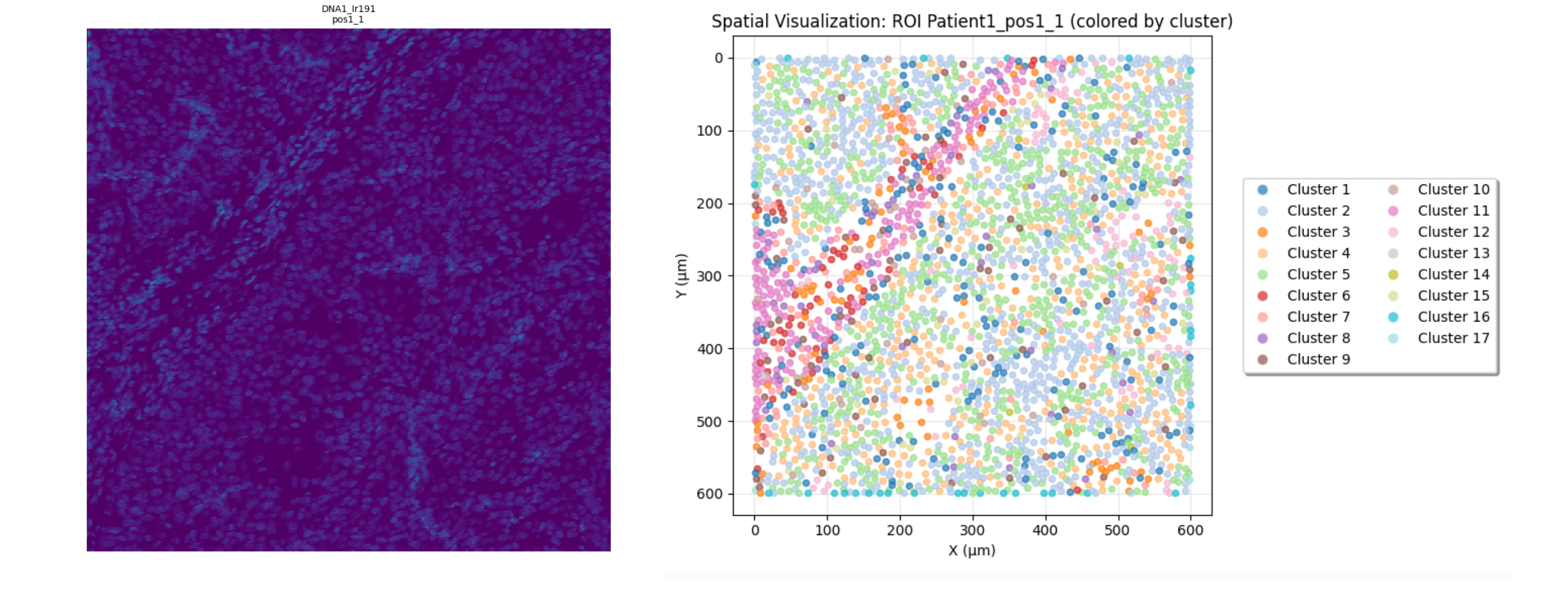
Figure 10: Spatial Visualizations in the Simple Analysis Window.
More Analyses and Features in OpenIMC
This quickstart covers the essential workflow to get you started with OpenIMC. However, the application includes many additional features and advanced analysis options to support a wide range of IMC experiments.
Additional Features:
State Management: Save and load complete analysis sessions for reproducibility and collaboration. States can be uploaded to Zenodo for publication. See State Management and Reproducibility for details.
Quality Control (QC): Tools for assessing image quality, detecting artifacts, and verifying segmentation accuracy.
Pixel Correlation Analysis: Explore channel relationships and spatial co-localization at the pixel level.
Advanced Spatial Analyses: Beyond the basics, the software supports expanded spatial statistics, neighborhood enrichment, proximity scores, and custom graph-building options.
Panel Design and Spillover Tools: Functions to assist with antibody panel QC and compensation for metal spillover.
Batch Processing, Automation, and Reports: Tools for end-to-end automated analysis, with exportable reports and visualizations.
We recommend exploring each section of the documentation after you have completed your first analysis to take full advantage of OpenIMC’s capabilities. The documentation provides detailed step-by-step usage guides, tips, and explanations for all analysis modules.